import tensorflow as tf
from tensorflow import keras

import numpy as np
import matplotlib.pyplot as plt
print(tf.__version__)
print(np.__version__)
2.11.0
1.21.5
fashion_mnist = keras.datasets.fashion_mnist


# 4개의 데이터 셋 반환(numpy 배열)
(train_images, train_labels), (test_images, test_labels) = fashion_mnist.load_data()
Downloading data from https://storage.googleapis.com/tensorflow/tf-keras-datasets/train-labels-idx1-ubyte.gz
29515/29515 [==============================] - 0s 0us/step
Downloading data from https://storage.googleapis.com/tensorflow/tf-keras-datasets/train-images-idx3-ubyte.gz
26421880/26421880 [==============================] - 4s 0us/step
Downloading data from https://storage.googleapis.com/tensorflow/tf-keras-datasets/t10k-labels-idx1-ubyte.gz
5148/5148 [==============================] - 0s 0s/step
Downloading data from https://storage.googleapis.com/tensorflow/tf-keras-datasets/t10k-images-idx3-ubyte.gz
4422102/4422102 [==============================] - 1s 0us/step
print("학습용 데이터 : x: {}, y:{}".format(train_images.shape, train_labels.shape) )
print("테스트 데이터 : x: {}, y:{}".format(test_images.shape, test_labels.shape) )
학습용 데이터 : x: (60000, 28, 28), y:(60000,)
테스트 데이터 : x: (10000, 28, 28), y:(10000,)
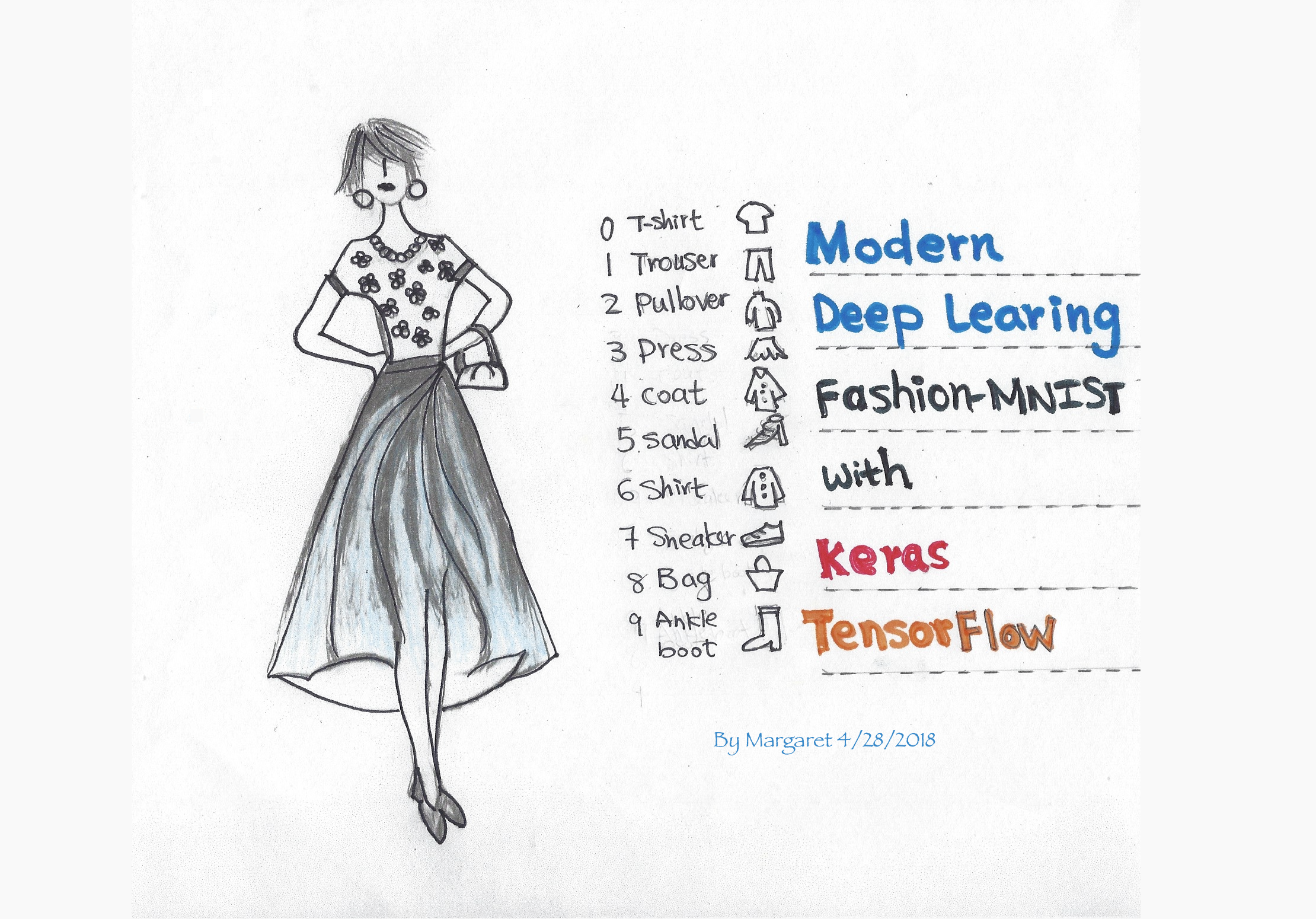
class_names = ['T-shirt/top', 'Trouser', 'Pullover', 'Dress', 'Coat',
               'Sandal', 'Shirt', 'Sneaker', 'Bag', 'Ankle boot']

print("학습용 데이터의 레이블 ", np.unique(train_labels) )
학습용 데이터의 레이블 [0 1 2 3 4 5 6 7 8 9]
plt.figure()
plt.imshow(train_images[0])   # 첫번째 이미지 데이터
plt.colorbar()     # 색깔 표시바
plt.grid(True)   # grid 선
plt.show()

fig = plt.figure(figsize=(20,15))

for i in range(25):
    ax = fig.add_subplot(5, 5, i+1, xticks=[], yticks=[])
    ax.imshow(train_images[i], cmap=plt.cm.binary)
    ax.set_xlabel(class_names[train_labels[i]], fontsize=16)

plt.show()

model = keras.Sequential([
    keras.layers.Flatten(input_shape=(28, 28)),
    keras.layers.Dense(128, activation='relu'),
    keras.layers.Dense(10, activation='softmax')
])

model.compile(optimizer='adam',
              loss='sparse_categorical_crossentropy',
              metrics=['accuracy'])
hist = model.fit(train_images, train_labels,
                 validation_data=(test_images, test_labels),
                 epochs=10, batch_size=32)
Epoch 1/10
1875/1875 [==============================] - 17s 9ms/step - loss: 3.1813 - accuracy: 0.6790 - val_loss: 0.7955 - val_accuracy: 0.7122
Epoch 2/10
1875/1875 [==============================] - 17s 9ms/step - loss: 0.6757 - accuracy: 0.7405 - val_loss: 0.6648 - val_accuracy: 0.7465
Epoch 3/10
1875/1875 [==============================] - 14s 8ms/step - loss: 0.5903 - accuracy: 0.7852 - val_loss: 0.7310 - val_accuracy: 0.7202
Epoch 4/10
1875/1875 [==============================] - 13s 7ms/step - loss: 0.5519 - accuracy: 0.8057 - val_loss: 0.5648 - val_accuracy: 0.8068
Epoch 5/10
1875/1875 [==============================] - 14s 7ms/step - loss: 0.5353 - accuracy: 0.8138 - val_loss: 0.6124 - val_accuracy: 0.7947
Epoch 6/10
1875/1875 [==============================] - 15s 8ms/step - loss: 0.5173 - accuracy: 0.8188 - val_loss: 0.5226 - val_accuracy: 0.8235
Epoch 7/10
1875/1875 [==============================] - 13s 7ms/step - loss: 0.5104 - accuracy: 0.8216 - val_loss: 0.5949 - val_accuracy: 0.8075
Epoch 8/10
1875/1875 [==============================] - 12s 6ms/step - loss: 0.4942 - accuracy: 0.8261 - val_loss: 0.5689 - val_accuracy: 0.8183
Epoch 9/10
1875/1875 [==============================] - 11s 6ms/step - loss: 0.4882 - accuracy: 0.8302 - val_loss: 0.5149 - val_accuracy: 0.8274
Epoch 10/10
1875/1875 [==============================] - 13s 7ms/step - loss: 0.4934 - accuracy: 0.8277 - val_loss: 0.5982 - val_accuracy: 0.7978
test_loss, test_acc = model.evaluate(test_images,  test_labels, verbose=2)

print('\n테스트 정확도:', test_acc)
313/313 - 1s - loss: 0.4957 - accuracy: 0.8347 - 1s/epoch - 3ms/step

테스트 정확도: 0.8346999883651733
loss = hist.history['loss']
val_loss = hist.history['val_loss']

epochs = range(1, len(loss) + 1)

plt.plot(epochs, loss, 'b--', label='Training loss')
plt.plot(epochs, val_loss, 'o-', label='Validation loss')
plt.title('Training and validation loss')
plt.xlabel('Epochs')
plt.ylabel('Loss')
plt.legend()

plt.show()

plt.clf()   # 그래프를 초기화합니다

acc = hist.history['accuracy']
val_acc = hist.history['val_accuracy']

plt.plot(epochs, acc, 'b--', label='Training acc')
plt.plot(epochs, val_acc, 'r', label='Validation acc')
plt.title('Training and validation accuracy')
plt.xlabel('Epochs')
plt.ylabel('Accuracy')
plt.legend()

plt.show()

# 테스트 세트에서 이미지 하나를 선택합니다
img = test_images[0]
print(img.shape)

# 이미지 하나만 사용할 때도 배치에 추가합니다
img = (np.expand_dims(img,0))
print(img.shape)
(28, 28)
(1, 28, 28)
np.set_printoptions(precision=8, suppress=True)
predictions_single = model.predict(img)
print(predictions_single)

idx = np.argmax(predictions_single[0])
print(idx)
print(class_names[idx])
1/1 [==============================] - 0s 34ms/step
[[0.         0.         0.         0.         0.         0.03429338
  0.         0.14071567 0.00000008 0.82499087]]
9
Ankle boot
import os

path = os.path.join(os.getcwd(), "dl_model")
savefile = os.path.join(path, "my_model_fashion.h5"  )

model.save(savefile)
!dir dl_model
 D 드라이브의 볼륨: BackUp
 볼륨 일련 번호: 4EB1-0AD7

 D:\GitHub\DeepLearning_Basic_Class\dl_model 디렉터리

2022-11-21  오후 04:30    <DIR>          .
2022-11-21  오후 04:30    <DIR>          ..
2022-11-21  오후 04:30         1,247,056 my_model_fashion.h5
               1개 파일           1,247,056 바이트
               2개 디렉터리  250,602,049,536 바이트 남음
# 모델을 불러온다.
load_model = keras.models.load_model(savefile)
load_model
<keras.engine.sequential.Sequential at 0x225651b23a0>
load_model.evaluate(test_images, test_labels, verbose=2)
313/313 - 1s - loss: 0.5982 - accuracy: 0.7978 - 783ms/epoch - 3ms/step
[0.598209023475647, 0.7978000044822693]